Source file: literate-basics.fut

Basic use of literate Futhark

The futhark literate command translates Futhark programs to Markdown files. Specially formatted comments, called directives, are replaced with executing parts of the program. The purpose of literate Futhark is to write small example programs with quick visualisations and such.

For example, let us define a function for generating a linearly spaced vector:

def linspace (n: i64) (start: f64) (end: f64) : [n]f64 =
  tabulate n (\i -> start + f64.i64 i * ((end - start) / f64.i64 n))

With an evaluation directive, we can show what it evaluates to:

> linspace 10i64 0f64 10f64

[0.0, 1.0, 2.0, 3.0, 4.0, 5.0, 6.0, 7.0, 8.0, 9.0]

> linspace 10i64 5f64 10f64

[5.0, 5.5, 6.0, 6.5, 7.0, 7.5, 8.0, 8.5, 9.0, 9.5]

If you look at the source file, you’ll see that that the results are not part of what I wrote. Those are automatically inserted by futhark literate.

The expressions in the directives are run by the Futhark interpreter (meaning they are slow), but any references to entry points (functions declared with entry) invoke compiled code. The Futhark part of a a literate Futhark program is compiled like an ordinary Futhark program, but only explicitly indicated entry points run fast.

Some values are boring when viewed as arrays of numbers.

def linspace_2d n start end : [n][n](f64, f64) =
  map (\x -> map (\y -> (x, y)) (linspace n start end))
      (linspace n start end)

entry spirals n v : [n][n]f64 =
  let f (x, y) = f64.sgn (f64.cos (f64.sqrt (x ** 2 + y ** 2)))
  in map (map f) (linspace_2d n (-v) v)

For expressions with an appropriate type, futhark literate can convert them to an image:

> :img spirals 200i64 30f64

Two-dimensional arrays of floats are interpreted as greyscale. A two-dimensional array of 32-bit integers is interpreted in RGB format.

entry colours n v : [n][n]u32 =
  let f (x, y) =
    (u32.f64 (x * y) & 0xFF) << 16
    | (u32.f64 (x + y) & 0xFF) << 8
    | (u32.f64 (f64.cos x - f64.sin y) & 0xFF)
  in map (map f) (linspace_2d n (-v) v)

This is more colourful.

> :img colours 200i64 30f64

Using the :img directive, we can draw whatever we want. However, if we just want to plot the value of some function, it would be pretty awkward to implement graphing every time.

def xys f n start end : ([n]f64, [n]f64) =
  unzip (map (\x -> (x, f x)) (linspace n start end))

entry plot_sqrt = xys f64.sqrt
entry plot_sin = xys f64.sin
entry plot_cos = xys f64.cos
entry plot_inv = xys (1 /)

The :plot2d directive lets us to a quick plot of pairs of x and y value arrays.

> :plot2d plot_sqrt 1000i64 0f64 100f64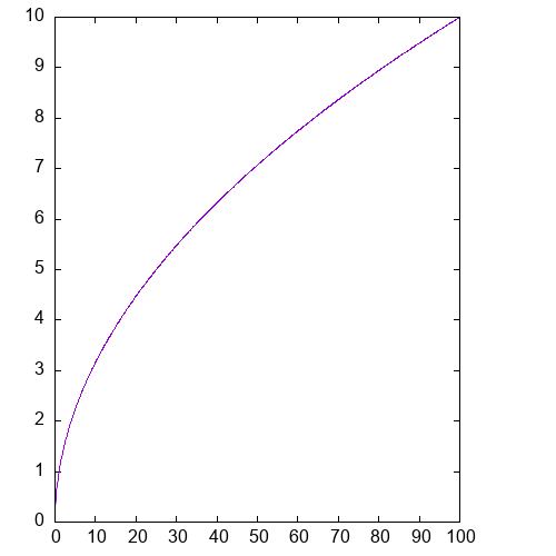

And if we want multiple plots in the same graph, then we pass a record of such pairs.

> :plot2d {sqrt=plot_sqrt 1000i64 0f64 25f64,
           sin=plot_sin 1000i64 0f64 25f64,
           cos=plot_cos 1000i64 0f64 25f64,
           inv=plot_inv 1000i64 1f64 25f64}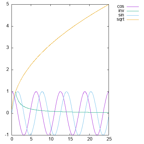

The :plot2d directive shells out to Gnuplot. For advanced needs, such as 3D plotting, we can write the Gnuplot commands ourselves.

entry plot3d n start end : ([]f64, []f64, []f64) =
  let f (x, y) =
    let z = f64.sin (5 * x) * f64.cos (5 * y) / 5
    in (x, y, z)
  in unzip3 (flatten (map (map f) (linspace_2d n start end)))

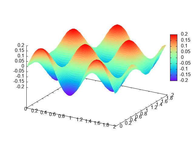
We pass in the data as a a record, and each field becomes a Gnuplot variable that contains the name of a data file.

> :gnuplot {ourdata=plot3d 100i64 0f64 2f64};
set palette rgbformulae 33,13,10
set dgrid3d 100,100
splot ourdata u 1:2:3 with pm3d notitle

Basic use of literate Futhark

See also